library(dplyr)
library(kableExtra)罕见病疫苗有效性样本量估计
我们首先导入后面会用到的包,后续会用到的dplyr的%>%管道函数和的kableExtra输出表格[1,2]。
疫苗有效性(Vaccine Efficacy)
当我们检验一款新的疫苗是否有效时,通常会使用疫苗有效性\(\pi\)(Vaccine Efficacy)这个指标。让\(P_1\), \(P_2\)分别为安慰剂组和接种疫苗组的发病率;\(N_1\), \(N_2\)分别为安慰剂组和接种疫苗组的群体总数;\(X, Y\)分别为安慰剂和疫苗组的病例人数。则\(X \overset{i.i.d}{\sim}\text{Binomial}(N_1, P_1)\), \(Y \overset{i.i.d}{\sim}\text{Binomial}(N_2, P_2)\)。
疫苗有效性为: \[ \pi = 1-(P_2/P_1) \tag{1}\] 原假设和备择假设为:
\[ H_0: \pi \leq \pi_0 \text{ versus } \ H_1:\pi>\pi_0 \tag{2}\]
如果一个疾病发病率较低,我们就需要更多受试者参加实验,在这种情况下\(X, Y\)可以被近似成为独立的泊松分布, 也就是\(X \overset{i.i.d}{\sim}\text{Poisson}(\lambda_1)\), \(Y \overset{i.i.d}{\sim}\text{Poisson}(\lambda_2)\) with \(\lambda_1 = N_1\cdot P_1, \lambda_2 = N_2\cdot P_2\).
\(Y\)给定\(T\)的条件概率分布为 \[ Y|T \sim \text{Binomial}(T, \theta)=\binom{T}{k} \theta^k(1-\theta)^{T-k} \text{ with } T = X + Y, \theta = \frac{\lambda_1}{\lambda_1+\lambda_2} \tag{3}\] 此时原假设和备择假设为:
\[ H_0: \theta \geq \theta_0 \text{ versus } \ H_1:\theta<\theta_0 \text{ where } \theta_0 = \frac{1-\pi_0}{2-\pi_0} \tag{4}\]
计算的P value 公式为 \[ p = \Pr[Y \leq Y_{\text{obs}} \mid Y \sim \text{Binomial}(T, \theta_0)] = \sum_{k=0}^{Y_{\text{obs}}} \binom{T}{k} \theta_0^k (1 - \theta_0)^{T - k} \tag{5}\]
计算Statistical power公式为 \[ 1 - \beta = \Pr[Y \leq Y_c \mid Y \sim \text{Binomial}(T, \theta_1)] = \sum_{k=0}^{Y_c} \binom{T}{k} \theta_1^k (1 - \theta_1)^{T - k} \tag{6}\]
计算临床实验所需样本量公式为 \[ N_2 = T/[(2-\pi_1)/P_1] \tag{7}\]
计算样本量所需的变量为\(\pi_0, \pi_1, \alpha\), 期望统计功效(1-\(\beta\))和安慰剂组发病率(\(P_1\))。
R代码示例
exact_conditonal_test <- function(T, alpha, power, theta0, theta1) {
  Y_c <- qbinom(alpha, size = T, prob = theta0)-1
  p_value <- pbinom(Y_c, size = T, prob = theta0)
  power <- pbinom(Y_c, size = T, prob = theta1)
  return(c(T, Y_c, power, p_value))
}

ect_sample_size <- function(T, pi0, pi1, incidence, alpha, power){
  theta0 <- (1-pi0) / (2-pi0)
  theta1 <- (1-pi1) / (2-pi1)
  table_t <- as.data.frame(do.call(rbind,
                               lapply(T, exact_conditonal_test,
                                      alpha = alpha, theta0= theta0, theta1 = theta1)),
                           .name_repair = "unique")
  colnames(table_t) <- c('T', 'Y_c', 'power', 'p-value')

  for (n in 1:nrow(table_t)){
    if (table_t$power[n] >= power && all(table_t$power[n:nrow(table_t)] >= power)) {
      min_n <- table_t$T[n]
      break
    }
  }
  result <- list(
    T_table = table_t,
    T = min_n,
    text = paste0('The min value of T achieve power of ', power, ' is ', min_n)
  )
  class(result) <- 'result'
  result
}

T2N <- function(T_value, incidence, pi1, dropout_rate){
  N2 <- T_value/((2-pi1)*incidence)/(1-dropout_rate)
  cat('The sample of vaccine group considering the drop out rate:', N2)
}
例1
[3] 在其论文中详细阐述了exact conditional方法的理论推导,并提供了不同样本量下统计功效(power)与显著性水平(significance level)的对应表格。为验证该方法的计算准确性,我们可以调用ect_sample_size()函数进行实证分析。具体参数设置:病例范围33到40,\(\pi_0=0.2,\pi_1=0.8, P_1=0.006, \alpha=0.025\), 目标统计功效为95%。将这些参数输入函数后,即可获得相应的样本量估计结果。
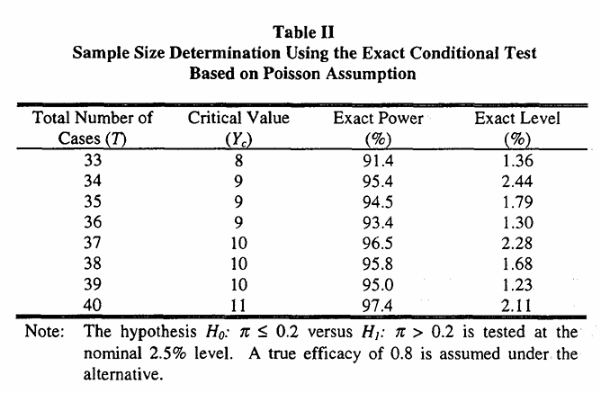
T <- 33:40 # the number of T
pi0 <- 0.2 # null hypothesis efficacy
pi1 <- 0.8 # True efficacy under alternative hypothesis
alpha <- 0.025 # type I error
incidence <- 0.006 # placebo incidence rate
power <- 0.95
res1 <- ect_sample_size(T, pi0, pi1, incidence, alpha, power)
kbl(res1$T_table)%>%
kable_styling(bootstrap_options = "striped", full_width = F, position = "left")| T | Y_c | power | p-value |
|---|---|---|---|
| 33 | 8 | 0.9139690 | 0.0136117 |
| 34 | 9 | 0.9540856 | 0.0244451 |
| 35 | 9 | 0.9449925 | 0.0178969 |
| 36 | 9 | 0.9347919 | 0.0129998 |
| 37 | 10 | 0.9653937 | 0.0227940 |
| 38 | 10 | 0.9584044 | 0.0168288 |
| 39 | 10 | 0.9504998 | 0.0123313 |
| 40 | 11 | 0.9738542 | 0.0211901 |
代码中的incidence 就是\(P_1\), 其他参数与上面提及的保持一致。可以看到输出的表格中样本量,critical value, statistical power和p value与论文中的表格完全一致。我们打印出能够达到95% statistical power的病例数
res1$T[1] 37打印结果显示 T = 37,与论文中的结果一致。接下来,利用公式 Equation 7 计算疫苗组所需的样本量。为了方便重复使用,我将该计算过程封装成了函数 T2N()。
在本示例中,未考虑受试者脱落情况,因此将 dropout_rate 参数设为 0。计算结果显示,疫苗组的样本量应不少于 5138.889。将该值乘以 2,即可得出疫苗组与安慰剂组的总样本量应不少于 10277.78,进一后为 10278。
该结果与论文完全一致,说明我们的算法实现是正确的。
T2N(37, incidence, pi1, dropout_rate = 0)The sample of vaccine group considering the drop out rate: 5138.889HRV-三期
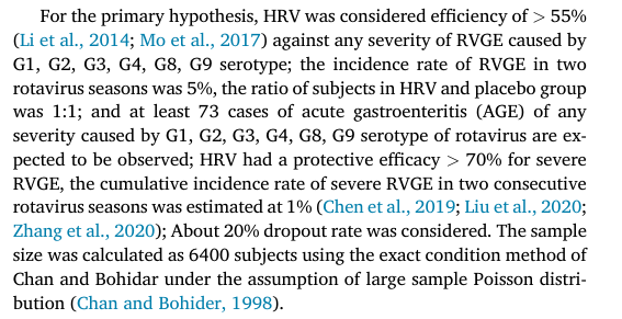
[5] 这篇论文原本是我们希望复现样本量计算的参考文献。然而在复现过程中发现,文中并未明确给出所需的关键参数 \(\pi_1\)、\(\alpha\) 以及期望的统计功效,因此无法准确计算所需样本量。因此,我们决定后续不再以该论文作为参考。
接下来的示例将以 HRV-三期这篇论文的参考文献为依据,该研究同样是关于轮状病毒(rotavirus)疫苗有效性的临床试验。
RV5
[6] 这篇论文将作为我们后续进行疫苗有效性检验样本量计算的参考文献。文中提供了以下参数:15% 的脱落率,(_0 = 0)、(_1 = 0.6)、(P_1 = 0.02)、显著性水平 (= 0.025),以及期望的统计功效为 80%。
代入上述参数后,可得所需的最小病例数为47。为了方便分组,我们取双数为48。接着,使用T2N()函数计算疫苗组所需的样本量,结果为至少2016.807,向上取整后为2020。该样本量结果与论文中的报告一致,验证了我们算法的正确性。
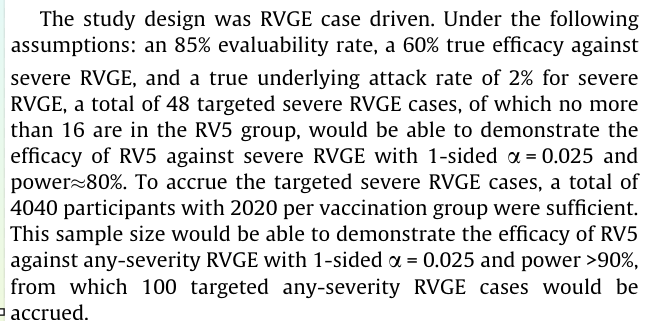
T <- 40:50 # the number of T
pi0 <- 0 # null hypothesis efficacy
pi1 <- 0.6 # True efficacy under alternative hypothesis
alpha <- 0.025 # type I error
incidence <- 0.02 # placebo incidence rate
power <- 0.8
res_rv5 <- ect_sample_size(T, pi0, pi1, incidence, alpha, power)
kbl(res_rv5$T_table)%>%
kable_styling(bootstrap_options = "striped", full_width = F, position = "left")| T | Y_c | power | p-value |
|---|---|---|---|
| 40 | 13 | 0.7692914 | 0.0192387 |
| 41 | 13 | 0.7363326 | 0.0137666 |
| 42 | 14 | 0.8052771 | 0.0217793 |
| 43 | 14 | 0.7757295 | 0.0157697 |
| 44 | 15 | 0.8362319 | 0.0243834 |
| 45 | 15 | 0.8100042 | 0.0178489 |
| 46 | 15 | 0.7819032 | 0.0129480 |
| 47 | 16 | 0.8396107 | 0.0199930 |
| 48 | 16 | 0.8146130 | 0.0146525 |
| 49 | 17 | 0.8650285 | 0.0221921 |
| 50 | 17 | 0.8429717 | 0.0164196 |
res_rv5$T[1] 47T2N(48, incidence, pi1, dropout_rate = 0.15)The sample of vaccine group considering the drop out rate: 2016.807PCV13
T <- 100:170 # the number of T
pi0 <- 0 # null hypothesis efficacy
pi1 <- 0.52 # True efficacy under alternative hypothesis
alpha <- 0.025 # type I error
incidence <- 0.0024 # placebo incidence rate
power <- 0.9
dropout <- 0.05
res_rv5 <- ect_sample_size(T, pi0, pi1, incidence, alpha, power)
kbl(res_rv5$T_table)%>%
kable_styling(bootstrap_options = "striped", full_width = F, position = "left")| T | Y_c | power | p-value |
|---|---|---|---|
| 100 | 39 | 0.9327041 | 0.0176001 |
| 101 | 40 | 0.9482422 | 0.0230220 |
| 102 | 40 | 0.9398983 | 0.0185334 |
| 103 | 41 | 0.9539240 | 0.0241168 |
| 104 | 41 | 0.9463670 | 0.0194790 |
| 105 | 41 | 0.9379379 | 0.0156509 |
| 106 | 42 | 0.9521763 | 0.0204360 |
| 107 | 42 | 0.9445280 | 0.0164733 |
| 108 | 43 | 0.9573873 | 0.0214036 |
| 109 | 43 | 0.9504577 | 0.0173077 |
| 110 | 44 | 0.9620567 | 0.0223810 |
| 111 | 44 | 0.9557870 | 0.0181532 |
| 112 | 45 | 0.9662365 | 0.0233675 |
| 113 | 45 | 0.9605713 | 0.0190093 |
| 114 | 46 | 0.9699746 | 0.0243623 |
| 115 | 46 | 0.9648618 | 0.0198753 |
| 116 | 46 | 0.9591042 | 0.0161360 |
| 117 | 47 | 0.9687057 | 0.0207504 |
| 118 | 47 | 0.9635009 | 0.0168941 |
| 119 | 48 | 0.9721463 | 0.0216341 |
| 120 | 48 | 0.9674468 | 0.0176618 |
| 121 | 49 | 0.9752232 | 0.0225259 |
| 122 | 49 | 0.9709847 | 0.0184387 |
| 123 | 50 | 0.9779725 | 0.0234250 |
| 124 | 50 | 0.9741539 | 0.0192242 |
| 125 | 51 | 0.9804271 | 0.0243311 |
| 126 | 51 | 0.9769904 | 0.0200179 |
| 127 | 51 | 0.9730892 | 0.0163948 |
| 128 | 52 | 0.9795269 | 0.0208191 |
| 129 | 52 | 0.9760104 | 0.0170934 |
| 130 | 53 | 0.9817936 | 0.0216276 |
| 131 | 53 | 0.9786270 | 0.0178000 |
| 132 | 54 | 0.9838175 | 0.0224427 |
| 133 | 54 | 0.9809686 | 0.0185143 |
| 134 | 55 | 0.9856234 | 0.0232641 |
| 135 | 55 | 0.9830627 | 0.0192358 |
| 136 | 56 | 0.9872337 | 0.0240913 |
| 137 | 56 | 0.9849340 | 0.0199641 |
| 138 | 57 | 0.9886687 | 0.0249240 |
| 139 | 57 | 0.9866051 | 0.0206989 |
| 140 | 57 | 0.9842415 | 0.0171178 |
| 141 | 58 | 0.9880963 | 0.0214398 |
| 142 | 58 | 0.9859725 | 0.0177687 |
| 143 | 59 | 0.9894263 | 0.0221865 |
| 144 | 59 | 0.9875194 | 0.0184261 |
| 145 | 60 | 0.9906117 | 0.0229385 |
| 146 | 60 | 0.9889008 | 0.0190897 |
| 147 | 61 | 0.9916676 | 0.0236957 |
| 148 | 61 | 0.9901338 | 0.0197592 |
| 149 | 62 | 0.9926077 | 0.0244576 |
| 150 | 62 | 0.9912335 | 0.0204342 |
| 151 | 62 | 0.9896509 | 0.0170053 |
| 152 | 63 | 0.9922139 | 0.0211146 |
| 153 | 63 | 0.9907943 | 0.0176055 |
| 154 | 64 | 0.9930874 | 0.0218000 |
| 155 | 64 | 0.9918148 | 0.0182114 |
| 156 | 65 | 0.9938653 | 0.0224901 |
| 157 | 65 | 0.9927253 | 0.0188226 |
| 158 | 66 | 0.9945576 | 0.0231847 |
| 159 | 66 | 0.9935370 | 0.0194390 |
| 160 | 67 | 0.9951735 | 0.0238835 |
| 161 | 67 | 0.9942604 | 0.0200603 |
| 162 | 68 | 0.9957211 | 0.0245863 |
| 163 | 68 | 0.9949046 | 0.0206862 |
| 164 | 68 | 0.9939581 | 0.0173403 |
| 165 | 69 | 0.9954782 | 0.0213166 |
| 166 | 69 | 0.9946308 | 0.0178995 |
| 167 | 70 | 0.9959886 | 0.0219512 |
| 168 | 70 | 0.9952305 | 0.0184634 |
| 169 | 71 | 0.9964426 | 0.0225898 |
| 170 | 71 | 0.9957646 | 0.0190318 |
res_rv5$T[1] 100T2N(156, 0.0024, 0.52, dropout_rate = dropout)The sample of vaccine group considering the drop out rate: 46230.44Reference
[1]
Wickham H, François R, Henry L, et al. Dplyr: A grammar of data manipulation [Internet]. 2023. Available from: https://dplyr.tidyverse.org.
[2]
Zhu H. kableExtra: Construct complex table with kable and pipe syntax [Internet]. 2024. Available from: http://haozhu233.github.io/kableExtra/.
[3]
Chan ISF, Bohidar NR. Exact power and sample size for vaccine efficacy studies. Communications in Statistics - Theory and Methods. 1998;27(6):1305–1322.
[4]
Loiacono MM. SAMPLE SIZE ESTIMATION AND POWER CALCULATIONS FOR VACCINE EFFICACY TRIALS FOR EXCEEDINGLY RARE DISEASES.
[5]
Wu Z, Li Q, Liu Y, et al. Efficacy, safety and immunogenicity of hexavalent rotavirus vaccine in Chinese infants. Virologica Sinica [Internet]. 2022 [cited 2025 Jul 22];37(5):724–730.
[6]
Mo Z, Mo Y, Li M, et al. Efficacy and safety of a pentavalent live human-bovine reassortant rotavirus vaccine (RV5) in healthy Chinese infants: A randomized, double-blind, placebo-controlled trial. Vaccine [Internet]. 2017 [cited 2025 Jul 22];35(43):5897–5904.